Replicating Sutton 1992
Written on
Replicating the Foundations: Sutton 1992 and the Alberta Plan
As I officially begin my D.Eng, I've been eager to start producing something. My method of learning has always been to understand things "under the hood". I don't feel I fully understand concepts until I can learn them from the ground up. To that end I've started working on a Python package "Alberta Framework" (alberta-framework) where I will work on replicating results from the foundational papers across the various steps of The Alberta Plan. I started with Pytorch but after reading some reddit posts on r/reinforcementlearning I stumbled across JAX. JAX is purpose built for high-performance computing and machine learning which lets you get a lot closer to a lower level language. Pytorch would have sufficed for early experiments, however given that I intend to build on this framework for the duration of my D.Eng I want to build on top of the best foundation for future work that will be a lot more computationally expensive.
I have started by setting up the main structure of the alberta-framework as a Python project that I'll likely publish on Pypi in the future. My first tests with the framework are to replicate the experiments in Sutton (1992).
Lab Environment
Right now I'm running experiments on my gaming PC. It's evident already that I'm going to need more compute in the not so distant future. Here's my setup for now:
Operating System: Debian Linux
GPU: NVIDIA RTX 3070 (8GB VRAM, 5,888 CUDA cores)
CPU: Intel i5-12400
Memory: 24GB RAM
Engineering the Foundation: JAX vs. PyTorch Benchmarks
My primary goal here was replicating the IDBD paper but I do want to build a solid foundation for future work so the framework is optimized when I get to more computationally expensive problems.
While I was building this I did a side test of the the paper experiments with alberta-framework (JAX) and a Pytorch implementation. The initial tests were discouraging when PyTorch blew JAX out of the water. However after learning how to properly use jax.lax.scan the benefits of JAX were obvious. As I understand it this is a bit of a rite of passage for people new to JAX.
- Throughput: JAX achieved a 2.78x speedup over eager PyTorch for the core IDBD update loops.
- Hardware Saturation: JAX demonstrated superior hardware engagement, maintaining an 11.47% average GPU utilization (reaching 79.0% peaks) while keeping CPU overhead remarkably low at 9.99%.
- Bottleneck Mitigation: The PyTorch implementation was heavily bottlenecked by host-side dispatch, consuming 40.24% CPU with minimal GPU engagement.
- XLA Compilation: The specialized kernel fusion provided by
jax.lax.scanallowed for a streamlined execution graph that is essentially a requirement for scaling to thousands of parallel agents.
So I will be continuing with JAX. To maintain the temporal uniformity required by the Alberta Plan while scaling the complexity of features, the performance gains provided by JAX's XLA compiler are indispensable.
The Problem: Non-Stationary Environments
Most machine learning assumes a stationary world where the relationship between inputs and targets is fixed. What attracted me to reinforcement learning and the Alberta Plan is that they're meant to address non-stationary, real-world problems.
Sutton’s 1992 paper introduced IDBD (Incremental Delta-Bar-Delta), an algorithm that automatically adjusts a vector of learning rates ($\alpha_i$), one for each input feature. It uses the gradient of the squared error to automatically increase the step-size for relevant features and silence the noise. IDBD addresses issues discussed in step 1 of the plan by "learning learning rates" so they don't have to be pre-programmed and can adapt to complex non-stationary environments.
The IDBD Algorithm
The following pseudocode represents the Incremental Delta-Bar-Delta (IDBD) algorithm as defined in Sutton (1992). This version manages a vector of learning rates by performing gradient descent on the log-step-size parameters ($\beta_i$).
Initialization: Initialize $h_i$ to $0$, and $w_i, \beta_i$ as desired for $i = 1, \dots, n$.
Main Loop: Repeat for each new example $(x_1, \dots, x_n, y^*)$:
- Generate Prediction: $y \leftarrow \sum_{i=1}^{n} w_i x_i$
- Calculate Error: $\delta \leftarrow y^* - y$
- Update Parameters for each $i = 1, \dots, n$:
- Meta-update (Adjust log-step-size): $\beta_i \leftarrow \beta_i + \theta \delta x_i h_i$
- Determine Step-size: $\alpha_i \leftarrow e^{\beta_i}$
- Weight Update (LMS/Delta Rule): $w_i \leftarrow w_i + \alpha_i \delta x_i$
- Memory Trace Update: $h_i \leftarrow h_i [1 - \alpha_i x_i^2]^+ + \alpha_i \delta x_i$
(where $[ \cdot ]^+$ denotes $\max(0, \cdot)$)
Experiment 1: The Tracking Problem
Experiment 1 in the paper tests the agent's ability to track a "moving target," learn relevant features, and discard irrelevant ones. The simulation for a non-stationary environment was a sum of five inputs, but every 20 examples, the sign of one input would flip (e.g., from +1 to -1).
This is a simple test of continual learning. If an agent ever stops learning or uses a learning rate that decays to zero, it will eventually fail as the environment shifts. An example in the alberta-framework successfully replicates Experiment 1 from Sutton (1992), demonstrating that IDBD maintains a high "readiness" to learn, identifying the shift and correcting the weights far faster than standard fixed-rate algorithms.
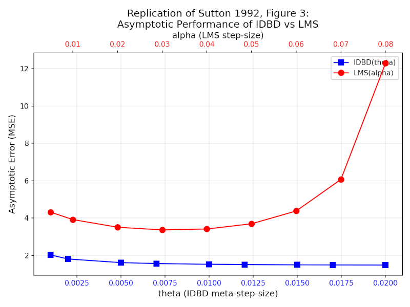
Figure 1: Performance comparison between IDBD and LMS.
Experiment 2: Does IDBD Find the Optimal Learning Rates?
Experiment 2 uses the same task as Experiment 1 but runs for 250,000 steps with a smaller meta-learning rate ($\theta = 0.001$) to observe the asymptotic behavior of the learned rates. This longer run demonstrates two key capabilities:
- Feature Selection: The agent must distinguish the 5 relevant inputs from the 15 irrelevant noise channels, driving the learning rates for noise toward zero.
- Optimal Convergence: The agent must converge to learning rates that minimize tracking error for the relevant inputs.
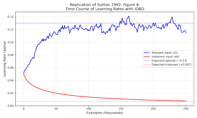
Figure 2: IDBD Learning Rate Adaptation (Signal vs. Noise).
Convergence and Optimality Analysis
After 250,000 steps, the IDBD algorithm effectively determined the optimal learning rate. The learning rates for the 15 irrelevant inputs were driven below 0.007—heading toward an asymptotic zero—while the learning rates for the 5 relevant inputs stabilized at $0.13 \pm 0.015$.
To verify if this stabilized value represents the true optimum, an empirical grid search was conducted. By fixing the irrelevant inputs' learning rates to zero and testing a range of fixed values for the relevant features, we can map the error surface. As shown in Figure 3, the resulting "U-shaped" curve reveals a clear performance minimum near $0.13 \pm 0.01$. This precisely matches the value discovered autonomously by IDBD, confirming that the algorithm successfully "learned the optimal learning rates" without human intervention.
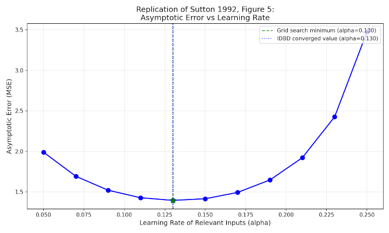
Figure 3: IDBD Convergence vs. Empirical Grid Search Minimum.
Results from the alberta-framework
Running the replication over 250,000 steps, the results were an almost exact match to the 1992 paper’s findings.
1. IDBD Outperforms LMS (Figure 1)
The example from the alberta-framework successfully demonstrates IDBD outperforms LMS as in Experiment 1 in Sutton (1992).
2. Learning Rate Evolution (Figure 2) The agent successfully performed "selective attention." The learning rates for the relevant inputs climbed to optimal levels (~0.13), while the irrelevant inputs were driven toward zero (<0.007).
3. The Asymptotic Error Curve (Figure 3) By running the same search over fixed learning rates that the experiment in the paper does, I generated the same "U-shaped" error curve. The IDBD algorithm converged at the minimum of this curve ($\alpha \approx 0.13$), proving it finds the optimal learning rate without manual tuning.
Why This Matters for the Alberta Plan
This replication validates the "Temporally Uniform" requirement of Step 1. The agent isn't "pre-trained"; it is continuously adapting its internal parameters.
In the Chronos-sec project I'm toying around with, I am applying this logic to honeypot logs. By using IDBD, I may be able to build a SOC agent that automatically learns which log features are currently predictive of a threat and which are background noise, without needing a human to re-engineer the feature set every time an attacker changes tactics.
Next Steps
I think I have a good handle on IDBD now and will move on to how Autostep (Mahmood et al., 2012) improves this by eliminating the meta-learning parameter ($ \theta $ in Sutton, 1992).
References
-
Sutton, R. S. (1992). Adapting bias by gradient descent: An incremental version of delta-bar-delta. Proceedings of the Tenth National Conference on Artificial Intelligence, 171-176.
-
Mahmood, A. R., Sutton, R. S., Degris, T., & Pilarski, P. M. (2012). Tuning-free step-size adaptation. 2012 IEEE International Conference on Acoustics, Speech and Signal Processing (ICASSP), 2121-2124. [DOI: 10.1109/ICASSP.2012.6288330]
-
Mahmood, A. R. (2010). Automatic step-size adaptation in incremental supervised learning (Master's thesis). University of Alberta, Edmonton, Canada.