Demonstrating Adaptive Step-Size Algorithm Needs External Normalization
Written on
Testing Real-World Data on IDBD and Autostep
My strategy for learning the foundations and contributing to the Alberta Plan for AI Research is to begin at Step 1 and work my way through the plan, learning and reading the associated literature as I go. This should give me a solid understanding of work to date and some experience in applying the main algorithms to real world problems. To that end I've implemented IDBD and Autostep in my Alberta Framework and began experimenting.
My early experiments with IDBD and Autostep on both synthetic tests and real SSH honeypot data are demonstrating that you most definitely need external normalization for stability. Autostep's internal normalization isn't enough and IDBD diverges almost immediately.
The Gap in Prior Work
In my post on replicating Sutton 1992, I replicated the experiments in Sutton 1992 showing that IDBD works exactly as advertised in the paper. However, real data and world experiences are more complex than the 1992 experiments.
In the type of data I'm interested in healthcare sensors, for example, span orders of magnitude (glucose: 70–400 mg/dL; patient counts: 0–thousands). Cybersecurity log sources can combine packet counts ($10^6$) with entropy scores (0–8). Step 1 of the Alberta Plan mentions that online normalization of the input data has yet to be tested and published so I set out to do that by collecting SSH attack data from a Cowrie honeypot over a few weeks and running that through the algorithms.
The Experiment
I tested four conditions:
| Condition | Optimizer | Normalization |
|---|---|---|
| IDBD | IDBD | None |
| IDBD + Norm | IDBD | OnlineNormalizer |
| Autostep | Autostep | None |
| Autostep + Norm | Autostep | OnlineNormalizer |
The OnlineNormalizer is a simple running mean/variance normalizer that standardizes features before they hit the learning algorithm. Nothing fancy, source code here.
I ran experiments on three synthetic streams with different types of scale non-stationarity:
- Abrupt scales — heterogeneous but static feature scales (log-spaced from $10^{-2}$ to $10^2$)
- Scale drift — scales follow a bounded random walk in log-space
- Scale shift — every 2,000 steps, each feature's scale is resampled from $[10^{-2}, 10^2]$
Then I validated on real data from chronos-sec, my SSH honeypot project collecting attack traffic from a VPS in Germany.
Results: Synthetic Benchmarks
First, as a test and comparison I ran on pre-normalized inputs (the Sutton 1992 benchmark) and IDBD wins. It converges about 10x faster than Autostep to the same asymptotic performance. Autostep eventually gets there and everything converges in after enough steps:
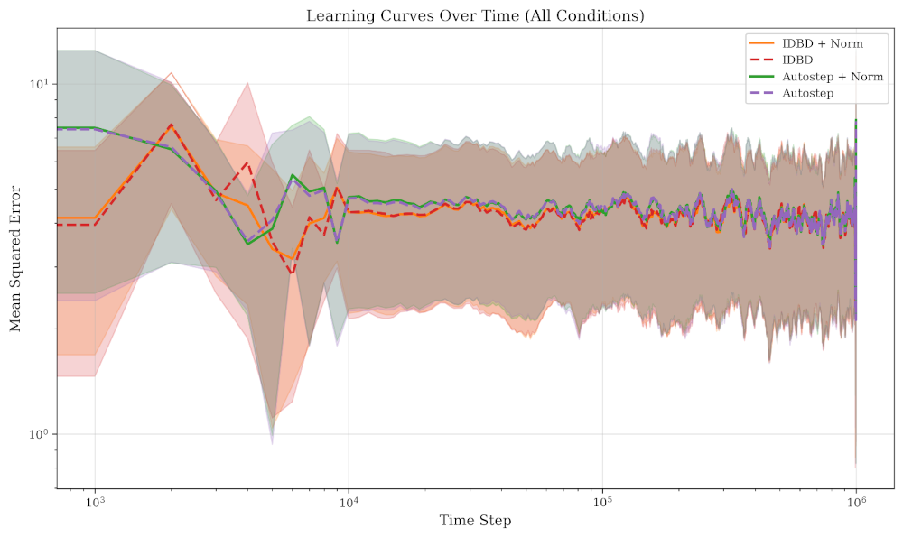
Figure 1: On pre-normalized inputs, IDBD converges faster. All methods reach the same final MSE (~1.46).
The picture changes completely when feature scales vary:
| Condition | Abrupt | Scale Drift | Scale Shift |
|---|---|---|---|
| Autostep + Norm | 0.11 | 0.13 | 0.14 |
| IDBD + Norm | 1.19 | 0.12 | NaN (diverged) |
| Autostep | 6.36 | 0.15 | 30.36 |
| IDBD | NaN | 0.27 | NaN |
IDBD diverges on 2 of 3 conditions without normalization. Even with normalization, it diverges on scale_shift. Autostep without normalization shows 30x higher MSE than with normalization on the hardest condition. Only Autostep + OnlineNormalizer achieves universally low error (0.11–0.14 MSE) across all conditions.
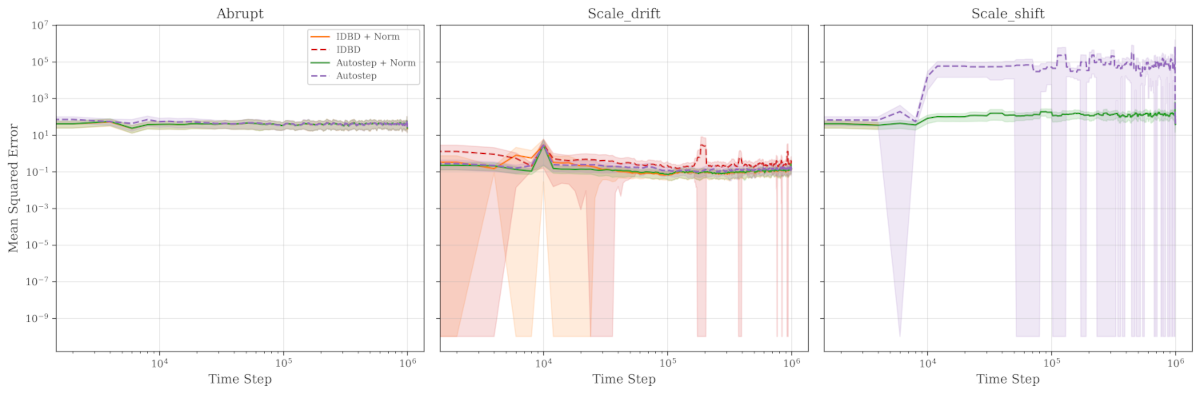
Figure 2: Learning curves broken down by non-stationarity type. Autostep + Norm (green) is the only method stable across all conditions.
The "Real" Test: SSH Honeypot Data
The synthetic benchmarks seem to prove external normalization is required but I wanted to test on real data. I wrote a little data collector chronos-sec that collects real attack traffic from a Cowrie SSH honeypot running in Germany. This honeypot has collected nearly 300k events over the course of a few weeks. Each session becomes a 17-dimensional feature vector with values spanning 8 orders of magnitude ($10^0$ to $10^8$):
| Index | Feature | Description | Scale Range |
|---|---|---|---|
| 0 | ip_reputation | Threat intel score | [0, 100] |
| 1 | country_risk | Country-based risk score | [0, 10] |
| 2 | connection_age | Seconds since first seen | [0, $10^6$] |
| 3 | auth_attempts | Failed authentication count | [0, 1000] |
| 4 | unique_users | Distinct usernames tried | [0, 500] |
| 5 | commands | Total commands executed | [0, 10000] |
| 6 | files_downloaded | Files retrieved | [0, 100] |
| 7 | lateral_attempts | Attempted pivots | [0, 50] |
| 8 | cmd_diversity | Shannon entropy of commands | [0, 8] |
| 9 | timing_randomness | Jitter in command timing | [0, 1] |
| 10 | encrypted | TLS/SSH encryption flag | {0, 1} |
| 11 | bytes_sent | Outbound data volume | [0, $10^8$] |
| 12 | bytes_received | Inbound data volume | [0, $10^8$] |
| 13 | hour_sin | sin(2π × hour/24) | [−1, 1] |
| 14 | hour_cos | cos(2π × hour/24) | [−1, 1] |
| 15 | day_sin | sin(2π × day/7) | [−1, 1] |
| 16 | day_cos | cos(2π × day/7) | [−1, 1] |
The reward function balances intelligence value against resource costs:
| Component | Value | Rationale |
|---|---|---|
| File download | +50 | High-value intelligence (malware samples, attack tools) |
| Credential capture | +20 | Useful for threat intelligence |
| Novel command | +5 | Each unique command reveals attacker TTPs |
| Duration cost | −0.1/sec | Longer sessions consume honeypot resources |
| Detection penalty | −30 | If attacker detects honeypot, session value drops |
Ground truth is computed using online 1-step TD(0) with terminal sessions. We predict total session value from the initial state, then observe the actual return with no bootstrapping:
$$\delta_t = r_t - \hat{V}(s_t; \mathbf{w}_t)$$
Running the four conditions on 276,403 observations from the honeypot:
| Condition | Valid Obs | First Divergence | Final 10k MAE |
|---|---|---|---|
| Autostep + Norm | 276,403 (100%) | Never | 0.73 |
| Autostep | 276,403 (100%) | Never | 11.01 |
| IDBD + Norm | 586 (0.2%) | Obs 587 | Diverged |
| IDBD | 24 (0.01%) | Obs 24 | Diverged |
IDBD diverges at observation 24. IDBD + Norm makes it to observation 587 before diverging. Autostep stays stable through all 276k observations, but with normalization achieves 15x lower error (0.73 vs 11.01 MAE).
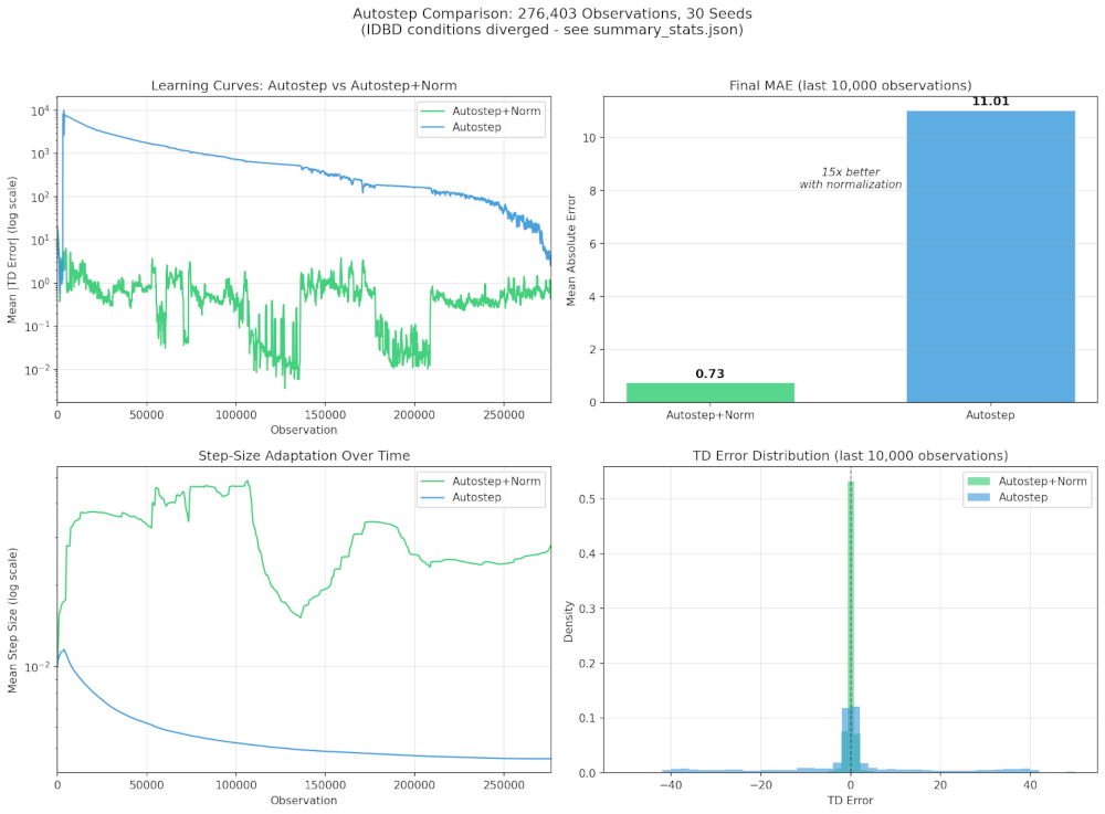
Figure 3: Four-panel summary of honeypot validation. Autostep + Norm achieves stable learning with 15x lower error than unnormalized Autostep. IDBD methods diverge within the first 600 observations.
The commands_count feature exhibited an 86x variance shift during the first coordinated attack wave — scale change magnitude that synthetic benchmarks don't capture. Real data is harder than synthetic benchmarks.
Findings
Using Autostep + OnlineNormalizer definitely performs better for continual learning on real-world data demonstrating the benefits of online normalization.
This is my first finding in my research and I hope to write it up as a paper after discussing more thoroughly with my advisor. It's not groundbreaking theory, but it's the kind of practical finding that I believe aligns with the Alberta Plan.
Why This Matters for the Alberta Plan
The Alberta Plan emphasizes learning from ordinary experience — not prepared datasets. The honeypot data is the kind of "ordinary experience" the Alberta Plan envisions: non-stationary, heterogeneous, noisy, with no human preprocessing the features into nice distributions. The finding that Autostep + OnlineNormalizer handles this robustly should be relevant to building practical continual learning systems.
Next Steps
I'm going to continue to work through the steps of the Alberta Plan adding to the framework as I go while I continue to learn and search for my dissertation topic. Right now I'm tackling cybersecurity problems because I'm most familiar with that data but I would like to look for applications in healthcare clinical operations like clinical decision support, pharmacy, labs or diagnostic imaging.
The alberta-framework now includes the synthetic experiments as reproducible examples. If you're working on similar problems, the code is available on PyPI or GitHub.
Experimental Details:
- 30 seeds per condition, 1M steps (synthetic) / 276k observations (honeypot)
- Hyperparameters: initial $\alpha$ = 0.1, meta rate = 0.01, normalizer decay = 0.99
- All experiments run on RTX 3070 using JAX +
jax.vmapfor batched execution
Lab Setup:
- OS: Debian Linux
- GPU: NVIDIA RTX 3070 (8GB VRAM, 5,888 CUDA cores)
- CPU: Intel i5-12400
- Memory: 24GB RAM
References:
- Sutton, R. S. (1992). Adapting bias by gradient descent: An incremental version of delta-bar-delta.
- Mahmood, A. R., Sutton, R. S., Degris, T., & Pilarski, P. M. (2012). Tuning-free step-size adaptation.
- Sutton, R. S., Bowling, M., & Pilarski, P. M. (2023). The Alberta Plan for AI Research.