Validating Streaming Deep RL on Attack Traffic
Written on
Validating Streaming Deep RL on Attack Traffic
I'm continuing to focus on RL prediction steps 1/2 of the Alberta Plan. In my first experiment, I showed that IDBD diverges almost immediately on the real honeypot data I'm collecting and testing with. Given enough time Autostep fared much better but needs external normalization to survive.
I'm interested in maximum performance for real time, continual learning. Exploring JAX a little more educated me on how vmap made multi-seed experiments practical on a single GPU.
I shared the post on my first experiments with Rupam Mahmood at University of Alberta and he pointed me to Elsayed et al. 2024 ("Streaming Deep Reinforcement Learning Finally Works") which I had not discovered yet and inquired if I had tested neural nets/non-linear learners. Elsayed et al. 2024 outlines a specific combination of techniques: observation-bounded gradient descent (ObGD), layer normalization (Ba et al. 2016), sparse initialization, and online data normalization using the algorithm from Welford 1962 to overcome the "stream barrier" that has historically prevented deep networks from learning in streaming RL settings. The results are exciting and were run on synthetic benchmarks: MuJoCo locomotion, MinAtar, and Atari. In my next set of experiments I set out to test whether the recipe will hold on actual adversarial, non-stationary data where the distribution shifts without warning. This led me into testing several combinations of non-linear learners with and without normalization and/or bounding. The non-linear architecture throughout is an MLP (multi-layer perceptron), a feedforward neural network with two hidden layers of 128 units each, LeakyReLU activations, and optionally parameterless LayerNorm applied before each activation. In the notation used below, MLP(128,128) refers to this architecture. Linear learners use a single dot product of weights and input features with no hidden layers, no activations.
Given one of my primary concerns is performance and the ability to run online agents on edge hardware I added support to the alberta-framework to start collecting system performance data during the experiment runs. The framework's learning loops originally returned only final learner state. I added two tracking systems:
- step-size tracking
StepSizeTrackingConfigrecords per-weight step-sizes at configurable intervals. I used this for testing Autostep's adaptive meta-parameters and IDBD's divergence behavior. - normalizer tracking
NormalizerTrackingConfigthat records per-feature running mean and variance, which enabled the reactive lag analysis that revealed how EMA and Welford normalizers respond to credential cannon bursts. Both record inside jax.lax.scan via conditional indexing, so they don't break JIT compilation or add control flow overhead. Every update now returns a metrics array with squared error, signed error, effective step-size, and (optionally) normalizer mean variance.
On the compute side, I added measure_compute_cost() to the experiment runner, which counts FLOPs per update using JAX's ahead-of-time compilation pipeline. The JIT-compiled update function is lowered to StableHLO (XLA's input language), then compiled for the target device, and the operation count is read from the compiled HLO graph via cost_analysis(). Combined with wall-clock timing (excluding JIT warmup via block_until_ready()) and JAX array memory accounting, this gives exact per-update FLOP counts, throughput in observations/second, and memory footprint. Note that the counts are device-specific: CPU and GPU XLA backends produce different HLO graphs due to different fusion and lowering decisions, so the numbers reported here are from the RTX 3070's compiled graph.
I'm up to 6 experiments total, testing 100 conditions, with 433,000 real attack observations (and growing) from the SSH honeypot. Here's what I found.
The Data
My Cowrie SSH honeypot running on a Linode VPS in Germany recorded ~433,000 sessions from roughly 4,050 unique IP addresses over 30 days (January 14 to February 12, 2026). The traffic is overwhelmingly automated:
| Category | Count | % of Traffic |
|---|---|---|
| Credential stuffers (1 auth attempt, disconnect) | ~377k | 96.7% |
| Scanners (connect, no auth) | ~12k | 3.1% |
| File downloaders | ~357 | 0.09% |
| Interactive (commands after login) | ~252 | 0.06% |
The top 10 IPs account for 57% of all traffic. Only 21 unique commands were observed across 1,740 total command executions. This is not a diverse dataset as it's dominated by bots.
Credential cannon campaigns
Three credential cannon bursts define the dataset's non-stationarity. Each dumps exactly 29,965 attempts in under two hours, then vanishes:
| Campaign | IP | Date | Observations | Duration |
|---|---|---|---|---|
| Cannon 1 | 172.239.19.112 | Jan 24 | 29,965 | 68 minutes |
| Cannon 2 | 146.190.228.30 | Jan 29 | 29,965 | 98 minutes |
| Cannon 3 | 172.239.28.137 | Feb 4 | 29,965 | 78 minutes |
These three IPs are almost certainly the same operator. Two share a /16 prefix (172.239.0.0/16) and all three are DigitalOcean IPs. They share the exact same session count 29,965 (likely a wordlist size), the same 1.1-second session duration, and the same recon command on their few successful logins:
uname -a && echo '---' && cat /etc/os-release && echo '---' && nproc && echo '---' && cat /etc/issue
They rotate IPs and repeat on a ~10-day cycle.
The DigitalOcean profiler botnet
357 file downloads came from 214 unique DigitalOcean IPs with zero reuse between weeks. Every download session follows the same script in under 3 seconds: log in, run a GPU-aware system profiler, download a payload, disconnect. The profiler checks for NVIDIA GPUs (lspci | grep -i nvidia), CPU model and core count, and fingerprints the coreutils implementation (cat --help, ls --help) — a known technique to distinguish real Linux from honeypot emulations like Cowrie's busybox. This operator is hunting for cryptomining-capable hosts.
The rare humans
Out of ~433,000 sessions, perhaps 5-10 showed signs of human activity. One ran history | tail -5 and free -h | head -2 — checking for previous activity. Another ran echo $((1337+1337)) — a honeypot detection technique, since emulated shells may not correctly evaluate arithmetic. A third checked /proc/1/mounts to determine if the target was a Docker container.
Why this data is hard for learning algorithms
Here are some of the properties that make this stream challenging:
-
Extreme non-stationarity: The credential cannon bursts inject ~30,000 near-identical observations (reward std = 0.002) into a stream that otherwise has high variance (reward std ~7.5). The data distribution shifts violently and without warning.
-
Heavy-tailed rewards: 95% of sessions earn +15 to +20. The rare +70 download sessions and -30 honeypot-detection sessions are sparse but important.
-
Temporal concentration: A single IP can generate 45x the normal observation rate for an hour, then disappear. Any algorithm with running statistics must handle these bursts without being permanently skewed.
Reward Function and Learning Setup
Each session earns a reward based on intelligence value minus resource costs:
| Component | Value | Trigger |
|---|---|---|
| File download | +50 | Attacker downloads a payload |
| New credentials | +20 | Any login attempt with a password |
| Novel commands | +5 each | Commands not seen in previous sessions |
| Duration cost | -0.1/sec | Prevents infinite sessions |
| Honeypot detected | -30 | Login + immediate disconnect, no activity |
The learning target is straightforward. All honeypot sessions are terminal, so there's no bootstrapping — the TD error is simply the prediction error on observed return:
$$\delta_t = r_t - \hat{V}(s_t; \mathbf{w}_t)$$
The 17 input features (auth attempts, command diversity, timing patterns, IP reputation, cyclical time encoding, etc.) are described in the autostep-normalization post. This work sits at Steps 1-2 of the Alberta Plan: continual supervised learning with given features (Step 1) and supervised feature finding via MLP hidden layers (Step 2).
The Journey: Six Experiments
Each experiment builds on the previous one's findings:
| Experiment | Question | Best MAE | Key Finding |
|---|---|---|---|
| 1 | Which optimizer survives? | 0.95 | Only Autostep+EMA is stable; IDBD diverges |
| 2 | Do MLPs help? | 0.68 | MLP(128,128)+EMA beats linear by 29% |
| 3 | Which normalizer? | 0.68 | EMA wins for MLPs, Welford for linear |
| 4 | LMS vs Autostep on MLP? | 0.67 | Tied; ObGD bounding matters more than optimizer |
| 5 | ObGD vs AGC bounding? | 0.68 | ObGD dominates; AGC fails on streaming data |
| 6 | Full technique ablation | 0.18 | Full Elsayed stack works on real data |
"Everything Diverges" — Experiment 1
This is the experiment from my autostep-normalization post. I found an error in the original implementation so this was re-run with the Autostep rewrite in v0.7.3 of the framework (self-regulated EMA normalizers matching Mahmood et al. 2012).
| Condition | Stable? | Diverges At | Final MAE |
|---|---|---|---|
| Autostep+EMA | Yes | — | 0.95 |
| Autostep (no norm) | No | obs 3,046 | — |
| IDBD+EMA | No | obs 555 | — |
| IDBD (no norm) | No | obs 17 | — |
One out of four conditions survives. IDBD's meta-learning rule is too aggressive for heavy-tailed, non-stationary rewards. Even Autostep without normalization diverges with the proper implementation from the paper.
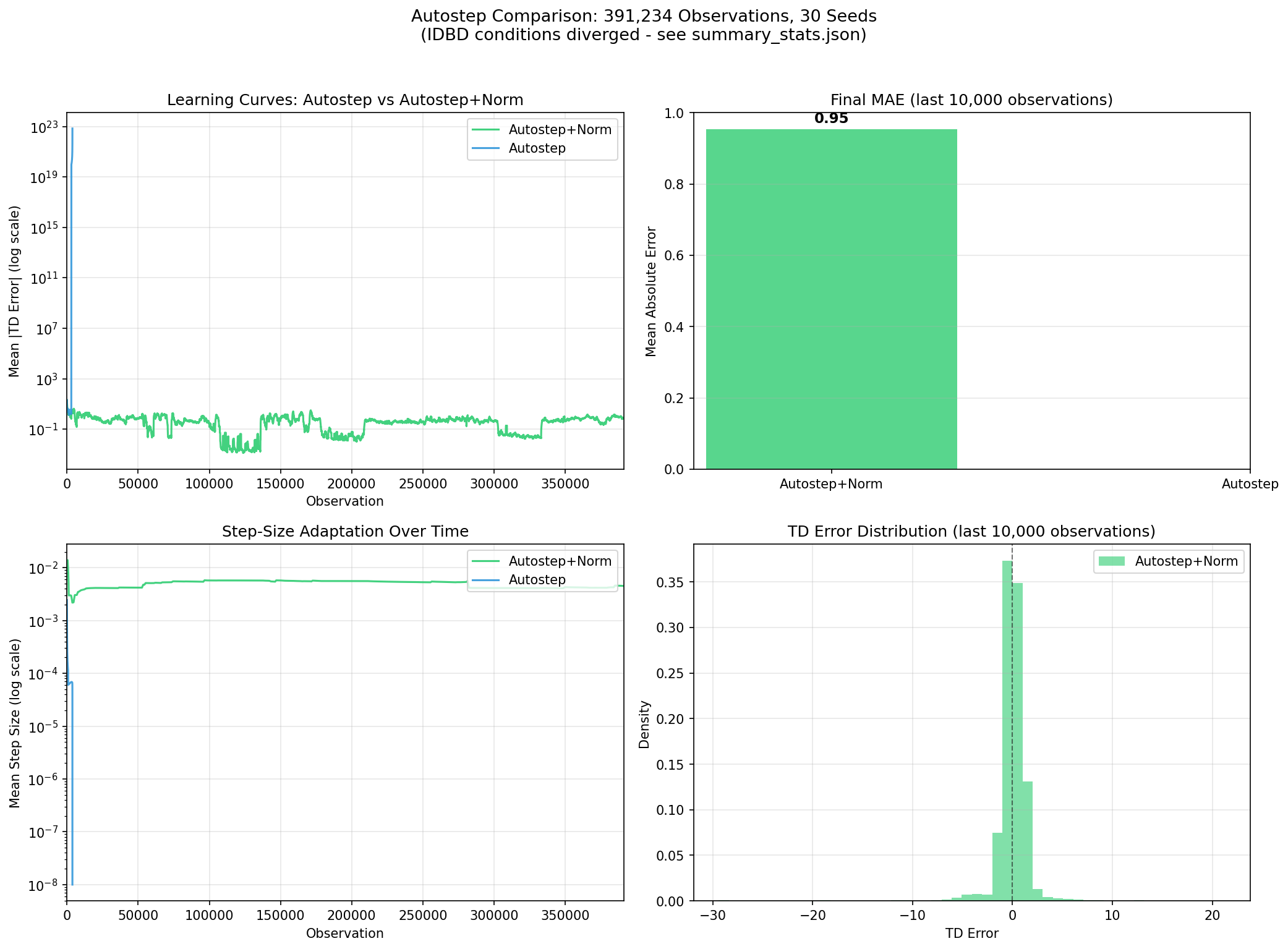
Autostep + EMA is the only stable condition. IDBD methods diverge within the first 600 observations.
My takeaway: normalization is not an optimization. It is a prerequisite for stability on this data.
"Bot Burst Recovery" — Experiment 3: EMA vs Welford
Elsayed et al. 2024 uses Welford's online algorithm (their Algorithms 4-6) for normalization. Welford computes cumulative mean and variance, giving equal weight to all past observations. I also tested EMA (exponential moving average), which exponentially forgets old statistics.
The question: does the paper's normalizer choice hold up on this non-stationary data?
| Learner | EMA Final MAE | Welford Final MAE | Winner |
|---|---|---|---|
| MLP(128,128) | 0.68 | 0.81 | EMA |
| MLP(128) | 0.77 | 0.78 | EMA (barely) |
| SGD+ObGD (linear) | 1.00 | 0.90 | Welford |
| Autostep (linear) | 0.95 | 0.86 | Welford |
The answer depends on architecture. EMA wins for MLPs; Welford wins for linear learners.
The mechanism ties directly to the credential cannon campaigns. When a burst dumps 30,000 near-identical observations into the stream, both normalizers adapt their statistics to the burst's narrow distribution. After the burst ends, the normalizer must re-adapt. EMA (decay=0.99) exponentially forgets the burst within a few hundred observations. Welford's cumulative statistics, now weighted by 30,000 identical observations, take much longer to reflect the post-burst distribution. EMA is working well for these simple SSH sessions that are terminal but I assume it will not perform well when I move to non-terminal sessions and eligibility traces.
For MLPs, where internal LayerNorm already handles activation scale, the input normalizer's main job is tracking the current distribution so EMA's forgetting is a clear advantage. For linear learners, Welford's stability during normal operation outweighs its slower recovery after bursts.
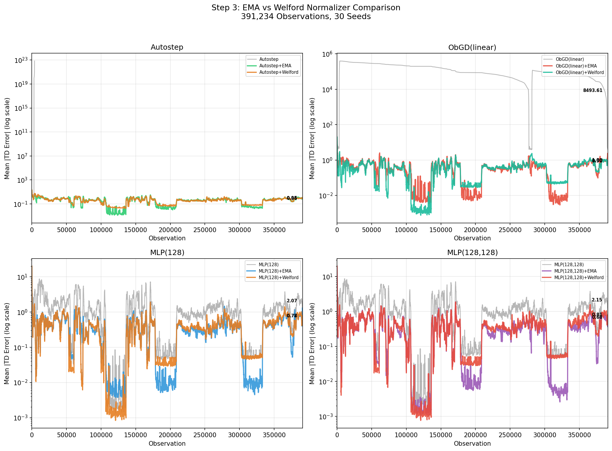
EMA recovers faster after credential cannon bursts. The advantage is clearest on the two-layer MLP (0.68 vs 0.81).
This is one place where our results diverge from the paper's choices. Elsayed et al. 2024 uses Welford throughout, which makes sense for their synthetic benchmarks where the data distribution is relatively stationary compared to real attack traffic. On our data, EMA is the better choice for MLPs.
Experiment 4: LMS vs Autostep on MLP
With EMA established as the normalizer for MLPs, I turned to the optimizer question: does Autostep's per-weight step-size adaptation improve over plain LMS (fixed step-size SGD) when both use ObGD bounding? I also tested whether ObGD bounding is necessary for each optimizer, and whether larger networks help.
Does Autostep improve over LMS on MLP?
| Optimizer | MLP(128,128) | MLP(256,256) | MLP(128,128,128) |
|---|---|---|---|
| LMS+ObGD+EMA | 0.68 | 0.69 | 0.71 |
| Autostep+ObGD+EMA | 0.69 | 0.67 | 0.68 |
Essentially tied. The differences are within noise across all architectures.
Is ObGD bounding necessary?
| With ObGD | Without ObGD |
|---|---|
| LMS+ObGD+MLP+EMA: 0.68 | LMS+MLP+EMA: 3.43 |
| Autostep+ObGD+MLP+EMA: 0.69 | Autostep+MLP+EMA: 0.76 |
- For LMS: absolutely. Without ObGD, LMS experiences catastrophic instability, the overall MAE reaches $10^{15}$ before the network eventually recovers to a mediocre 3.43 final MAE.
- For Autostep: barely. Without ObGD, Autostep still achieves 0.76 — worse than with bounding but still reasonable.
The ObGD bounding ratio reveals the mechanism: 1.0 for LMS (every single update is throttled) vs 0.0 for Autostep (no updates are throttled). LMS at step_size=1.0 always overshoots without ObGD's constraint. Autostep's per-weight adaptive step-sizes naturally self-regulate, making the bound redundant.
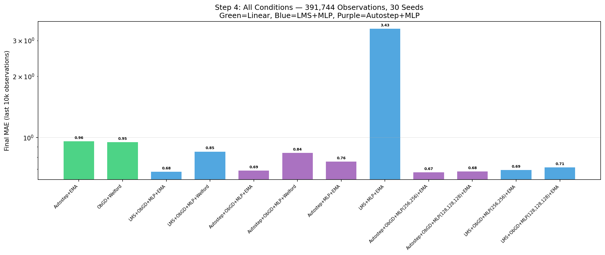
LMS without ObGD (blue, center) explodes to 3.43 MAE. Autostep without ObGD (purple) stays at 0.76. With ObGD, both optimizers are tied at 0.68-0.69.
Does more capacity help? No. MLP(128,128), MLP(256,256), and MLP(128,128,128) all fall in the 0.67-0.71 range. The 17-dimensional input doesn't have enough features to benefit from additional capacity.
Experiment 5: ObGD vs AGC
Adaptive Gradient Clipping (AGC) from Brock et al. 2021 clips gradients per-unit based on the ratio of parameter norm to gradient norm. It was designed for training large NFNets without batch normalization. ObGD (Elsayed et al. 2024, Algorithm 3) bounds a single global scalar, the effective step-size, based on the product of gradient magnitude and eligibility trace norm. I tested both on MLP(128,128) with EMA normalization.
| Condition | Final MAE | vs Baseline |
|---|---|---|
| LMS+ObGD+MLP+EMA | 0.68 | 0.71x |
| Autostep+ObGD+MLP+EMA | 0.69 | 0.72x |
| Autostep+MLP+EMA (no bounding) | 0.76 | 0.79x |
| Autostep+EMA (linear baseline) | 0.96 | 1.0x |
| Autostep+AGC(0.02)+MLP+EMA | 1.01 | 1.05x |
| LMS+AGC+MLP+EMA | 1.22 | 1.27x |
| LMS+MLP+EMA (no bounding) | 3.43 | 3.58x |
Every AGC condition is worse than ObGD — and most are worse than the linear baseline. The best AGC result (Autostep+AGC at clip_factor=0.02, MAE 1.01) barely matches the linear Autostep+EMA baseline.
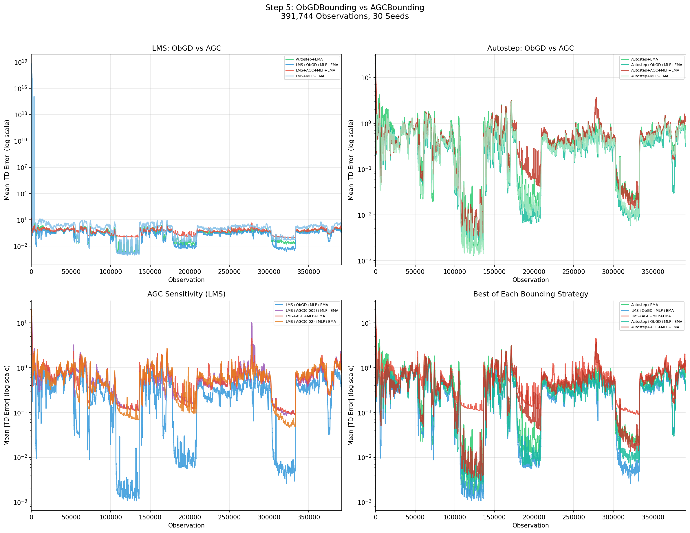
ObGD wins decisively. Every AGC condition underperforms the linear baseline.
I guess this is just a case of wrong tool for the job. The per-unit clipping introduces inconsistent updates creating a noisy, uncoordinated learning signal. ObGD's global bound maintains gradient coherence: all units are scaled by the same factor, preserving the direction of the update while only reducing its magnitude.
AGC was designed for mini-batch training where per-unit gradient statistics are stable across the batch. In streaming RL with single-sample updates, the per-unit gradient norms are too noisy for reliable clipping decisions.
Experiment 2 is summarized in the progression table above — MLPs with ObGD bounding outperform linear learners (0.68 vs 0.95 MAE).
The Full Ablation: Experiment 6
Finally a full $2^4$ factorial ablation of {SparseInit, LayerNorm, ObGD, EMA} crossed with two optimizers (LMS, Autostep) on MLP(128,128). 32 MLP factorial conditions, plus 8 linear baselines and 15 hyperparameter sensitivity sweeps. 55 conditions total, 30 seeds each, on ~433,000 observations.
Deviations from Elsayed et al. 2024: Based on Experiment 3, I substitute EMA for the paper's Welford normalizer. I omit the paper's reward scaling (their Algorithm 5) since our reward distribution is bounded and dominated by the +20 credential bonus. I also omit eligibility traces ($\lambda=0$) since all honeypot sessions are terminal ($\gamma=0$), whereas the paper uses $\lambda=0.8$ with $\gamma=0.99$ throughout. I'll get to that later as I continue building the stack and collecting more advanced data.
Top Results
| Rank | Condition | Final MAE |
|---|---|---|
| 1 | MLP+LMS+Sparse+LN+ObGD+EMA | 0.18 |
| 2 | MLP+LMS+Sparse+LN+ObGD | 0.20 |
| 3 | MLP+LMS+LN+ObGD+EMA | 0.20 |
| 4 | MLP+AS+Sparse+LN+ObGD+EMA | 0.21 |
| 5 | MLP+LMS+Sparse+ObGD+EMA | 0.21 |
| — | Linear+AS+Welford (best linear) | 0.37 |
| — | Linear+ObGD+EMA | 0.38 |
The full LMS technique stack achieves 0.18 MAE — a dramatic improvement over the 0.68 from Experiments 2-5. The jump comes from adding SparseInit and LayerNorm, which weren't part of the earlier experiments. Notably, the top three conditions are all LMS — with the full stack in place, LMS outperforms Autostep (0.18 vs 0.21).
The "winning pipeline"
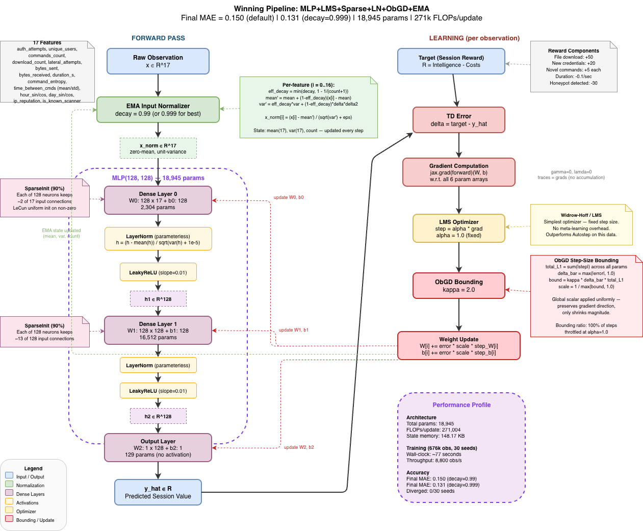
Which Techniques Matter
Each optimizer has one technique it depends on for survival, and the two optimizers depend on different ones:
-
LMS needs ObGD. Without ObGD bounding, LMS diverges unless LayerNorm is present as a fallback. This is consistent with the paper's finding that ObGD removal causes the "largest effect on performance." We saw this directly in Experiment 4 — LMS without ObGD explodes to $10^{15}$ MAE before recovering to a mediocre 3.43.
-
Autostep needs EMA. Without EMA normalization, Autostep diverges unless LayerNorm is present. This is consistent with every previous experiment and with the Elsayed et al. finding that removing normalization left the agent "no longer able to improve its performance."
-
LayerNorm is a universal fallback stabilizer. It prevents divergence in configurations that would otherwise be lost, but with degraded accuracy — LMS+LayerNorm without ObGD survives at 1.63 MAE, Autostep+LayerNorm without EMA survives at 0.31 MAE. When the full stack is present, LayerNorm contributes to the best result (0.18 MAE).
-
SparseInit has negligible effect on its own but matters through its interaction with LayerNorm (see below).
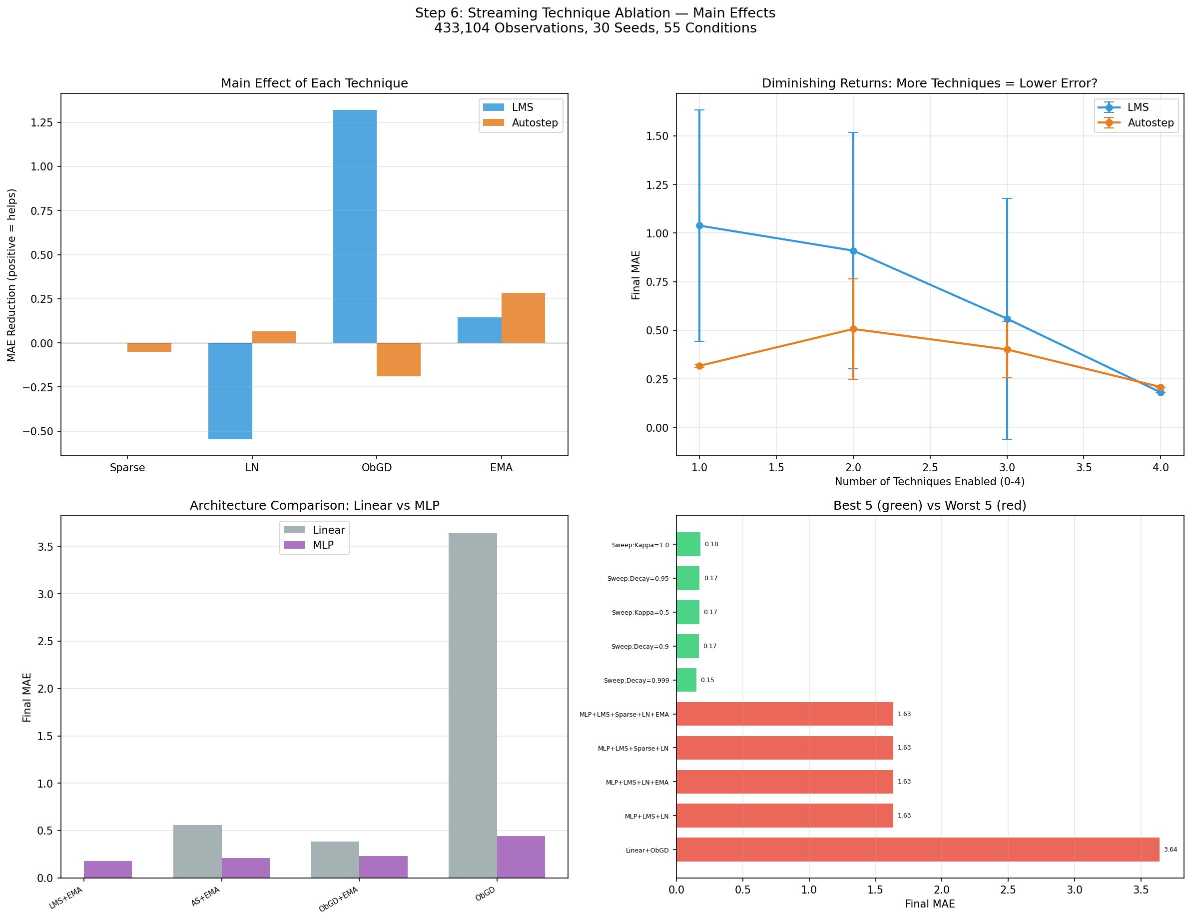
Each optimizer depends on a different technique. ObGD is critical for LMS; EMA is critical for Autostep. LayerNorm acts as a fallback stabilizer for both.
How Techniques Interact
Some technique pairs work better together than you'd expect from their individual contributions (synergy), while others overlap and provide diminishing returns (redundancy):
ObGD + EMA: strong synergy. They address orthogonal failure modes — ObGD prevents step-size explosions, EMA prevents feature scale drift. Together they're much better than either alone. This is the strongest interaction in the ablation, especially for Autostep.
SparseInit + LayerNorm: synergy. Sparse initialization (90% zero weights) creates dead neurons. LayerNorm rescales activations to keep all neurons contributing. Together they prevent the "dying ReLU" problem while maintaining initialization diversity. Neither helps much alone.
LayerNorm + EMA: redundancy. Both normalize activations, so combining them provides diminishing returns. This is expected — they're doing overlapping work.
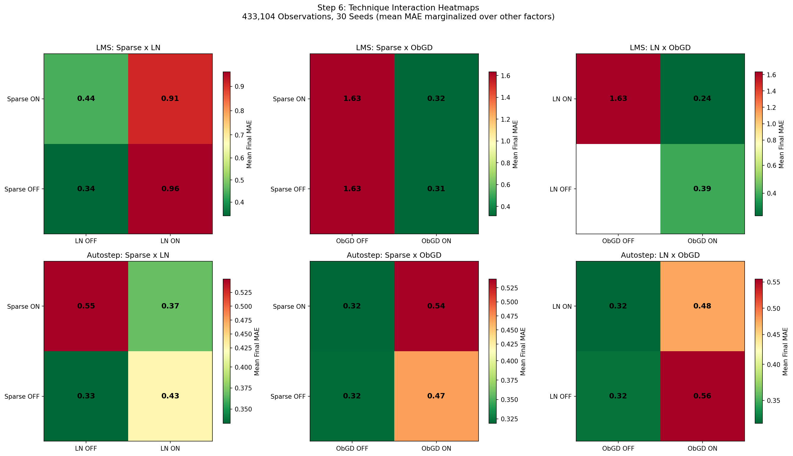
Warm colors = redundancy (techniques overlap). Cool colors = synergy (techniques complement each other).
Divergence and Hyperparameters
12 of 55 conditions diverged. The pattern reveals that each optimizer needs at least one stabilizer:
- LMS without both ObGD and LayerNorm diverges (obs 3-256). Either ObGD or LayerNorm alone can prevent divergence, but without both, LMS is unstable. LayerNorm alone stabilizes the model but with degraded accuracy (~1.63 MAE).
- Autostep without both EMA and LayerNorm diverges (obs 3,043-3,064). Either EMA or LayerNorm alone can prevent divergence. LayerNorm alone achieves ~0.31 MAE — better than LMS without ObGD, reflecting Autostep's superior self-regulation.
- No condition with both ObGD and EMA diverges, regardless of optimizer.
On hyperparameters, I swept the full-stack configuration across several ranges.
Autostep tau was insensitive across four orders of magnitude. Mahmood et al. 2012 noted that Autostep's performance was "not strongly dependent on $\tau$" and recommended setting it to the expected number of data samples needed for learning. Our sweep confirms this and extends the finding to a wider range than the original paper tested (they used $\tau=10^4$ on all problems without sweeping).
| $\tau$ | Final MAE |
|---|---|
| 100 | 0.207 |
| 1,000 | 0.211 |
| 10,000 (default) | 0.208 |
| 100,000 | 0.207 |
| 1,000,000 | 0.206 |
Sparsity — insensitive. Dense initialization (0.0) is marginally worse but still works. The Elsayed default of 0.9 is fine.
| Sparsity | Final MAE |
|---|---|
| 0.0 (dense) | 0.197 |
| 0.5 | 0.186 |
| 0.7 | 0.181 |
| 0.9 (default) | 0.180 |
| 0.95 | 0.183 |
EMA decay — insensitive for final accuracy, but decay rate affects adaptation speed. Slower decay (0.999) achieves the best final MAE but adapts more slowly initially, resulting in higher overall error across the full stream.
| Decay | Final MAE | Overall MAE |
|---|---|---|
| 0.9 | 0.168 | 0.263 |
| 0.95 | 0.175 | 0.270 |
| 0.99 (default) | 0.180 | 0.315 |
| 0.999 | 0.150 | 0.366 |
ObGD kappa — mildly sensitive. Tighter bounding (lower $\kappa$) outperforms the paper's default on our heavy-tailed reward distribution.
| $\kappa$ | Final MAE |
|---|---|
| 0.5 | 0.171 |
| 1.0 | 0.180 |
| 2.0 (default) | 0.180 |
| 4.0 | 0.183 |
| 8.0 | 0.197 |
Computational Cost: Can You Deploy This?
If we want to deploy this agent on edge hardware or something like a syslog server collecting log data, compute budget matters. The agent is going to have to process observations faster than they arrive, ideally on modest hardware. I measured FLOPs by lowering each learner's update function through JAX's XLA compiler and reading the operation count from the compiled HLO graph via cost_analysis(). These are exact counts of the operations in the compiled program, not estimates.
| Configuration | Final MAE | FLOPs/Update | Throughput (obs/s) | Memory |
|---|---|---|---|---|
| MLP+LMS+All | 0.18 | 271,003 | 477,014 | 148 KB |
| MLP+AS+All | 0.21 | 934,343 | 200,395 | 370 KB |
| Linear+ObGD+EMA | 0.38 | 460 | 2,750,666 | 0.3 KB |
The optimizer — not the stability techniques — dominates compute cost. Autostep requires 3.4x more FLOPs than LMS while achieving worse accuracy (0.21 vs 0.18 MAE). The reason is straightforward: LMS (Widrow & Hoff 1960) does one multiply-accumulate per weight ($\mathbf{w} \leftarrow \mathbf{w} + \alpha \delta \mathbf{x}$). Autostep does that plus maintains a separate adaptive step-size for every weight, a running normalizer for each step-size, and an overshoot check that scales all step-sizes down if the total update would be too large (Mahmood et al. 2012, Equations 4-7). That's multiple extra passes over every weight on every update.
For this task, LMS is the clear winner: better accuracy at 3.4x fewer FLOPs. But this is terminal prediction as every session ends and the target is a known reward. Once I move to non-terminal sessions with bootstrapping ($\gamma > 0$) and eligibility traces ($\lambda > 0$), the learning problem is going to get harder. The target becomes a moving estimate, traces propagate credit across time steps, and the optimizer has to track a shifting value function rather than just fit observed returns. Autostep's per-weight adaptation may earn back its 3.4x compute overhead in that setting. We'll find out.
Marginal cost of each technique
| Technique | Marginal FLOPs (LMS) | % of Total |
|---|---|---|
| SparseInit | 0 | 0.0% |
| EMA normalizer | +261 | 0.1% |
| LayerNorm | +7,858 | 2.9% |
| ObGD bounding | +75,607 | 27.9% |
SparseInit is free, it only affects weight initialization (Algorithm 1 in Elsayed et al.), not the update computation. EMA costs almost nothing (261 FLOPs, 0.1%) for the most universally important technique in the stack. ObGD is the most expensive at 27.9% of total FLOPs, but it's the technique that prevents LMS from diverging: it computes the bound $M = \alpha \kappa \bar{\delta} |\mathbf{z}_w|_1$ and scales the step-size: $\alpha \leftarrow \min(\alpha/M, \alpha)$ on every update.
MLP vs linear: the 589x gap
The best MLP requires 589x more FLOPs than the best linear learner. In exchange, it achieves 2.1x better accuracy (0.18 vs 0.38 MAE). For context: at 271,003 FLOPs per update, the MLP processes one observation in ~2.1 $\mu$s on an RTX 3070 (477k obs/s JIT-compiled). Even the peak credential cannon rate (~7.3 obs/s at peak) is trivially within budget. The linear model at 460 FLOPs would handle any traffic rate on any hardware.
To put these numbers in deployment terms: a minimal SSH session (TCP handshake, SSH key exchange, one auth attempt, disconnect) is roughly 4 KB on the wire. That's the dominant session type (96.7% of our traffic). At different network bandwidths, assuming the link is saturated with nothing but SSH credential stuffing:
| Link Speed | Sessions/s | MLP Headroom | Linear Headroom |
|---|---|---|---|
| 10 Mbps | ~280 | 1,700x | 9,800x |
| 100 Mbps | ~2,800 | 170x | 980x |
| 1 Gbps | ~28,000 | 17x | 98x |
Yes, a 1 Gbps link saturated entirely with minimal SSH sessions is an absurd scenario and would imply 28,000 concurrent attackers each completing a session every second. However even then, the MLP has 17x headroom and the linear model nearly 100x. Our actual peak traffic (credential cannon) hit 7.4 sessions/second. A realistic large-scale honeypot deployment might see 100-1,000x that; the learner is never the bottleneck. The honeypot software itself (Cowrie's Twisted event loop, TCP state tracking, log I/O) would saturate long before either model breaks a sweat.
Three deployment configurations cover the spectrum:
| Use Case | Configuration | FLOPs | MAE | Memory |
|---|---|---|---|---|
| Best accuracy | MLP+LMS+Sparse+LN+ObGD+EMA | 271,003 | 0.18 | 148 KB |
| Balanced | MLP+LMS+Sparse+ObGD+EMA | 263,145 | 0.21 | 148 KB |
| Edge/embedded | Linear+ObGD+EMA | 460 | 0.38 | 0.3 KB |
The Recipe (so far)
The best configuration for streaming prediction on non-stationary honeypot data:
- Optimizer: LMS (step_size=1.0) — outperforms Autostep at 3.4x fewer FLOPs
- Bounding: ObGD ($\kappa=2.0$, or $0.5$ for heavy-tailed domains) — limits effective step-size per update
- Network: MLP(128, 128) with parameterless LayerNorm, LeakyReLU, 90% sparse init
- Normalizer: EMA (decay=0.99) — exponential forgetting adapts to distribution shift
- No eligibility traces — all honeypot sessions are terminal ($\gamma=0$)
This achieves 0.18 MAE on 433k real observations which is 2.1x better than the best linear learner and 5.3x better than the Experiment 1 baseline. Zero divergence across 30 seeds.
My Learnings
Every optimizer diverges without normalization. IDBD diverges in 17 observations, Autostep in 3,046. I expected normalization to help. I didn't expect it to be the difference between learning and not learning.
The optimizer matters less than the techniques. Once bounding and normalization are in place, LMS achieves 0.18 MAE and Autostep 0.21. Mahmood et al. 2012's Autostep was designed specifically for the problem of tuning-free step-size adaptation — and it delivers on that promise. But on MLPs with ObGD bounding, the fixed step-size LMS is actually slightly better, at 3.4x fewer FLOPs. The ObGD bound from Elsayed et al. (Algorithm 3) effectively does the step-size adaptation that Autostep would otherwise provide.
AGC is the wrong tool here. Adaptive gradient clipping from Brock et al. 2021 was designed for batch training of NFNets. I tested it as an alternative to ObGD hoping its per-unit approach might offer finer-grained control. Instead, every AGC condition was worse than the linear baseline. The per-unit clipping that works well with mini-batches creates too much noise on single-sample updates.
Autostep's tau is insensitive across four orders of magnitude. From $\tau=100$ to $\tau=1{,}000{,}000$, MAE stays at approximately 0.21. Mahmood et al. 2012 suggested that performance was "not strongly dependent on $\tau$". The sweep on real non-stationary data confirms this emphatically. This is exactly the kind of robustness you want in a deployed system.
The Elsayed defaults transfer from synthetic to real data. Sparsity (0.9), kappa (2.0), architecture (128, 128) all work at their published defaults. The one modification I needed is the normalizer: EMA instead of the paper's Welford algorithm, because EMA recovers faster from the credential cannon bursts that define our dataset's non-stationarity. All tested decay rates (0.9-0.999) achieve strong final accuracy.
Next Steps
I'm still getting my head around all the components of RL architecture and how they fit together. These experiments are as much a learning experience for me as an attempt to answer some questions from the papers using real attack data.
Everything in this post is Steps 1-2 of the Alberta Plan: continual supervised learning (Step 1) and supervised feature finding via MLP hidden layers (Step 2). All honeypot sessions are terminal ($\gamma=0$), so every target is an observed return — there's no bootstrapping. The TD error $\delta_t = r_t - \hat{V}(s_t)$ is just a prediction error on known outcomes.
The next move is Step 3 (Prediction I): continual GVF prediction learning with bootstrapping. This means shifting from terminal session-level predictions to within-session, step-by-step TD learning where $\gamma > 0$ and targets include the agent's own value estimates: $\delta_t = r_t + \gamma \hat{V}(s_{t+1}) - \hat{V}(s_t)$. Bootstrapping introduces a new source of instability — the target is now a moving estimate, not ground truth — and the stability techniques validated here will need to be re-tested in that setting. Eligibility traces ($\lambda > 0$) also become relevant; Elsayed et al. 2024 uses $\lambda=0.8$ throughout, which we omitted.
General Value Functions (GVFs) open up auxiliary predictions beyond session reward: predicting time until disconnect, probability of file download, or likelihood of lateral movement — each as a separate value function with its own cumulant and termination condition. These predictions could serve as features for higher-level decision-making, which is Step 4 (Prediction II): predictive feature finding.
Beyond prediction, the end goal is a deployed RL agent that selects actions, for example "observe", "engage", "tarpit", "redirect", "terminate" that will be capable of real-time defense. That's the control problem, and it builds on everything above.
For deployment, the linear model at 460 FLOPs per update can run on anything. The MLP at 271k FLOPs needs a real processor but fits in 148 KB of memory. Both options are viable for a VPS-hosted honeypot.
The alberta-framework and the chronos-sec code are both on GitHub.
Lab Setup:
- OS: Debian 13.3 (Trixie)
- GPU: NVIDIA RTX 3070 (8GB VRAM, 5,888 CUDA cores)
- CPU: Intel i5-12400 (6 cores, 12 threads)
- Memory: 24GB RAM
Experimental Details:
- 30 seeds per condition, ~433k observations from 26+ days of real attack traffic
- Rewards computed from session metadata: file downloads (+50), credentials (+20), novel commands (+5 each), duration cost (-0.1/sec), honeypot detection (-30)
- Framework: alberta_framework v0.7.3 (Experiments 1-5), v0.7.4 (Experiment 6) with JAX, vmap-batched across seeds on GPU
- Autostep uses self-regulated EMA normalizers ($\tau=10{,}000$) with overshoot prevention, following Mahmood et al. 2012
- Deviations from Elsayed et al. 2024: (1) EMA normalizer replaces Welford (based on Experiment 3), (2) reward scaling omitted (bounded reward distribution), (3) eligibility traces omitted ($\lambda=0$, terminal sessions)
- "Final MAE" is mean absolute error over the last 10,000 observations
References:
- Ba, J. L., Kiros, J. R., & Hinton, G. E. (2016). Layer normalization. arXiv:1607.06450.
- Brock, A., De, S., Smith, S. L., & Simonyan, K. (2021). High-performance large-scale image recognition without normalization. ICML.
- Elsayed, M., Vasan, G., & Mahmood, A. R. (2024). Streaming deep reinforcement learning finally works. arXiv:2410.14606.
- Mahmood, A. R., Sutton, R. S., Degris, T., & Pilarski, P. M. (2012). Tuning-free step-size adaptation. IEEE ICASSP.
- Sutton, R. S. (1992). Adapting bias by gradient descent: An incremental version of delta-bar-delta. AAAI.
- Sutton, R. S., Bowling, M., & Pilarski, P. M. (2022). The Alberta Plan for AI research. arXiv:2208.11173.
- Welford, B. P. (1962). Note on a method for calculating corrected sums of squares and products. Technometrics.
- Widrow, B., & Hoff, M. E. (1960). Adaptive switching circuits. IRE WESCON Convention Record.